


Up: Parent directry
Interferometry on a blazed grating
1
Daigo Tomono
February 4, 2002
Abstract:
Interferometric calculations are done on a flat blazed grating. It is
found that to maximize the efficiency,
- Order of diffraction
 must be as small as possible.
- Incident angle
 and emergent angle
  must be as
close as possible.
must be as
close as possible.
- Groove interval
 must be as big as possible.
to avoid shadowing. These parameters will be decided from the
physical limitation of production of the grating and assembly of the
spectrometer.
Secondary peaks beyond the first local minima has 4.7% peak intensity
of the primary peak. This is not considered in efficiency calculation.
For the  -band, calculated efficiency is more than about 96%
throughout the band when
-band, calculated efficiency is more than about 96%
throughout the band when
 ,
,  , and
, and
 . With larger , efficiency increases. When and
are separated, efficiency drops to about 95% for 20 deg
difference.
. With larger , efficiency increases. When and
are separated, efficiency drops to about 95% for 20 deg
difference.
When the slit width is wider than a certain limit, namely, spatial
resolution of the instrument is less than the diffraction limit of the
telescope, spectral resolution of the spectrometer is limited by the
geometrical size of the slit. When the field of view (FOV) of a
spatial element is  of diffraction limited spatial elements, we
need about
of diffraction limited spatial elements, we
need about  times more grating grooves to achieve the same spectral
resolving power for a diffraction limited instrument.
times more grating grooves to achieve the same spectral
resolving power for a diffraction limited instrument.
Postscript version of this report is also available:
grating.ps.gz.
Interferometry is calculated on a grating with groove interval and
groove angle  as in Figure 1.
Figure 1:
Geometry of light and blazed grating
|
|
Incident light from
 with signed angle comes
from distance
with signed angle comes
from distance  . Consider detecting emergent light with signed
angle at
. Consider detecting emergent light with signed
angle at
 distance
  . Here, light
reflected at the point
. Here, light
reflected at the point  is considered. Throughout this report,
refractive index of media around the grating is assumed to be 1.
is considered. Throughout this report,
refractive index of media around the grating is assumed to be 1.
Distance between  and
and  is
is
 and distance between and the coordinate origin is
 . So,
. So,  can be approximated as
 . Likewise
 .
Using the incident and emergent angles,
.
Using the incident and emergent angles,
 and
and
 . Therefore, light path going through can be
explained as
. Therefore, light path going through can be
explained as
 and
and
 .
.
On the th groove of total  grooves,
 and
and
 . Therefore, phase delay
 at
at  of the light from and reflected at
is
of the light from and reflected at
is
where
 .
Here, we define
.
Here, we define
 |
(3) |
and
![\begin{displaymath}
E=
\frac{1}{\cos \varepsilon}
(\sin [\alpha - \varepsilon] + \sin [\beta - \varepsilon])
\end{displaymath}](img59.png) |
(4) |
Using the equations, complex amplitude of the light detected at is
calculated from integration over the grating surface. Here we take the
shadowing effect into account. As shown in Figure 2, only
 of the groove surface reflects the light.
Figure 2:
Shadowing of the incident or emergent light on different
grating shapes.
![\includegraphics[scale=0.5]{shadow.eps}](img66.png) |
![\includegraphics[scale=0.5]{shadow_right.eps}](img67.png) |
| (a) |
(b) |
|
Normalizing at  and
and  , intensity of the light detected at
is
, intensity of the light detected at
is
![\begin{displaymath}
I(P_2) = \frac{1}{N^2}\frac{1-\cos[kNdA]}{1-\cos[kdA]}
\times \frac{2}{(kd'E)^2} (1-\cos[kd'E])
\end{displaymath}](img70.png) |
(8) |
The first term of Equation 8, which we call grating function
is from the periodical sum over the grooves of the grating which has
peaks at  so
so
 |
(9) |
When the incident angle and diffraction order is known,
emergent angle can be calculated as
![\begin{displaymath}
\beta = \arcsin[\frac{m\lambda}{d} - \sin\alpha]
\end{displaymath}](img73.png) |
(10) |
where is an integer of the diffraction order.
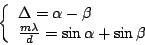
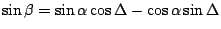
On the other hand, when we define difference of incident and emergent
angles,
 |
(11) |
and is calculated as follows with fixed :
![\begin{displaymath}
\alpha \mbox{,} \beta =
\arcsin\left[
\frac{ \frac{m\lamb...
...os\Delta)-(\frac{m\lambda}{d})^2}}
{2(1+\cos\Delta)}
\right]
\end{displaymath}](img75.png) |
(12) |
Derivation is described in Appendix A
The second term of Equation 8, which is called slit
function, is the diffraction from the grooves. This peaks at or
 |
(13) |
Distance from the peak to the first minima is almost at the same
interval that the first term has for the peaks on  .
.
When the entrance slit is narrow enough, Equation 8
can be used to asses properties of the output spectra. As shown below,
the slit can be treated narrow and  can be treated as
instrumental profile when difference of incident light direction (half
width)
can be treated as
instrumental profile when difference of incident light direction (half
width)  is smaller than
![$\sim \lambda /
(2Nd\cos[\alpha_0])$](img80.png) where
where  is the center direction of the
incident light. In Figure 3, left-most curve shows
normalized profile of at
is the center direction of the
incident light. In Figure 3, left-most curve shows
normalized profile of at  and
and  .
Horizontal axis is change of
.
Horizontal axis is change of  from the center of the
spectra.
from the center of the
spectra.
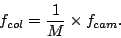
For  , spectral resolution of the grating is calculated as
follows. First, we have a peak at
, spectral resolution of the grating is calculated as
follows. First, we have a peak at
 for a
wavelength
for a
wavelength  . Near the peak, there are local minima at
 . We define spectral resolution when the next
spectral element of
. We define spectral resolution when the next
spectral element of  is at the local minima
  . Namely,
for the th order, we have a peak for at
. Namely,
for the th order, we have a peak for at
 . Thus, the wavelength difference
 or
or
 |
(14) |
or
 |
(15) |
Beyond the local minima, there are second local maxima near  that
makes
that
makes
![$\cos[kdNA'] = -1$](img96.png) beyond the first local minima. For the peak of
th order diffraction of
beyond the first local minima. For the peak of
th order diffraction of  ,
,
 .
The position corresponds to the peaks for
.
The position corresponds to the peaks for
 .
.
Near the secondary peaks, from , grating function is
assuming  .
.
Exact positions of secondary peaks can be obtained by taking
differential of the grating function. Position and value of the peaks
weakly depends on . The secondary peaks are nearer to the primary
peak and has intensity about 4.7 % of the primary peak when is more
than about 1000.
When the entrance slit is wide, Equation 8 has to be
integrated over the entrance slit, assuming that the light coming to
different locations on the entrance slit is not coherent. This results
in spectral resolution not being geometrically limited rather than being
diffraction limited as for a narrow entrance slit.
When the direction of the collimated light spreads from
 to
to
 ,
Equation 8 has to be integrated from
,
Equation 8 has to be integrated from  to
to
 and profile of the spectra can be assessed.
with
 .
We can assume
.
We can assume
 (slit width is
small, if not narrow) and
(slit width is
small, if not narrow) and  (the spectrometer is used around
the Bragg's condition). In the case,
(the spectrometer is used around
the Bragg's condition). In the case,
 and
and
![$1-\cos[kd'E]\sim(kd'E)^2/2$](img119.png) .
When the grating is used in the th order, can be replaced with
.
When the grating is used in the th order, can be replaced with
 . Near the and of spectra we
are observing,
. Near the and of spectra we
are observing,  . Therefore,
![$1-\cos[kdA] = 1-\cos[kdA'] \sim
(kdA)^2/2$](img122.png) . Here, we define
. Here, we define
![$A'_{1,2} = A_{1,2} - 2\pi m/(kd) \sim \sin
\alpha_0 + \sin\beta - 2\pi m/kd \pm \cos[\alpha_0] \delta\alpha$](img123.png) and
the integration becomes
and
the integration becomes
with
 and
and
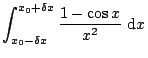
![$\delta x\equiv kNd\times\cos[\alpha_0] \delta\alpha$](img128.png) . The equation
cannot be integrated analytically.
. The equation
cannot be integrated analytically.
Figure 3 shows results from numerical integration of
Equation 26 with different  . For
smaller than
. For
smaller than  , width of the spectra is comparable with that
for
, width of the spectra is comparable with that
for  . On the other hand, for
 , the profile
gets half of the center at
, the profile
gets half of the center at
 .
.
Figure 3:
Numerical integration of Equation
26. From left to right, curves show
results for of 0, 2, 4, 6, 8, 10, and 12. Results are
normalized at  .
.
|
|
From the definition,
 corresponds to a threshold
angular half width of the slit
corresponds to a threshold
angular half width of the slit
![\begin{displaymath}
\delta\alpha_{th} \sim \pi/(kNd\cos[\alpha_0]) =
\lambda/(2Nd\cos[\alpha_0]).
\end{displaymath}](img135.png) |
(26) |
If the half width of the direction of the incident light onto the
grating is more than
 , spectral resolution of the
spectrometer is not limited by diffraction of the grating, but limited
by geometrical width of the slit.
, spectral resolution of the
spectrometer is not limited by diffraction of the grating, but limited
by geometrical width of the slit.
When the instrument is spatially diffraction limited at  ,
field of view (FOV) of a spatial element on a telescope with entrance
pupil diameter of
,
field of view (FOV) of a spatial element on a telescope with entrance
pupil diameter of  is in the order of
 .
Thus, the system
.
Thus, the system  becomes
 . On a
seeing limited instrument, FOV of a spatial element is more than for the
diffraction limited instrument. Here, we assume to observe FOV
times larger than that for a diffraction limited instrument. In the
case, system becomes
. On a
seeing limited instrument, FOV of a spatial element is more than for the
diffraction limited instrument. Here, we assume to observe FOV
times larger than that for a diffraction limited instrument. In the
case, system becomes
 .
.
When the diameter of the grating is  , beam width of incident
light becomes
, beam width of incident
light becomes
![$D_{gr}\cos[\alpha_0]$](img143.png) . Considering only about the beam in
the dispersion direction, solid angle of the light going into the
grating is
. Considering only about the beam in
the dispersion direction, solid angle of the light going into the
grating is
![$\Omega_{gr} \sim n^2\lambda_0^2\pi/(4
D_{gr}^2\cos[\alpha_0])$](img144.png) . Therefore, from
. Therefore, from  , half width of
the incident beam direction is
, half width of
the incident beam direction is
![\begin{displaymath}
\delta\alpha
\sim n\lambda_0/(2 D_{gr}\cos[\alpha_0]) \sim n \delta\alpha_{th}.
\end{displaymath}](img146.png) |
(27) |
For a seeing limited instrument, spectral resolution is limited by the
geometrical image size of the entrance slit, rather than the diffraction
of the grating.
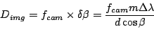
When the spectral resolution of the spectrometer is geometrically
limited, spectral resolving power is calculated as follows.
Half width  of the slit image for a certain wavelength in
the emergent light from the grating is
of the slit image for a certain wavelength in
the emergent light from the grating is
Therefore, from Equation 9, wavelength difference becomes
where  is the full width. Therefore spectral resolving
power becomes
is the full width. Therefore spectral resolving
power becomes
Comparing this with Equation 15, resolving power of the
spectrometer is degraded by a factor of
![$1/n\cos[\alpha_0]$](img160.png) for
for
 . As a consequence, we need
![$n\cos[\alpha_0]$](img162.png) times more
grooves for a seeing limited spectrometer to achieve the same spectral
resolving power as for a diffraction limited spectrometer.
times more
grooves for a seeing limited spectrometer to achieve the same spectral
resolving power as for a diffraction limited spectrometer.
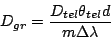
consideration
Spectral resolution of the spectrometer is considered from conservation
of . With telescope aperture diameter , width of the
slit on the sky  , square root of system is
 .
.
On the focal plane array (FPA), image of the slit has to be  .
Thus, with width of the light direction conversing to the FPA
.
Thus, with width of the light direction conversing to the FPA
 , focal ratio of the spectrometer camera is
Therefore, with focal length of spectrometer camera  diameter
of beam emerging from the grating is
diameter
of beam emerging from the grating is
 |
(39) |
and grating width is
 |
(40) |
Size of the image of the slit on the FPA is adjuste to be the same as
the size of a spectral element dispersed by the grating. From Equation
9, width of the beam direction of a spectral element
is
 |
(41) |
Therefore,
 |
(42) |
Putting Equation 43 into Equation 41,
 |
(43) |
and number of grating grooves illuminated by the beam is
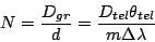 |
(44) |
With spectral resolution
 , number of
grooves becomes
, number of
grooves becomes
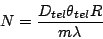 |
(45) |
Moreover, if slit FOV is times that of the
diffraction limit of the telescope
 ,
,
 |
(46) |
Design of a seeing limited spectrograph
Sometimes, we need to adjust dispersion so that a spectral element is
dispersed onto a disired size  , with the image size
  of the slit being different. For this kind of requirements, design steps
are considered here.
of the slit being different. For this kind of requirements, design steps
are considered here.
First we define required spectral resolving power
 with being full width of
wavelenght for a spectral element. Moreover, groove interval of the
grating and diffraction order , difference of incident angle and
emergent angle
with being full width of
wavelenght for a spectral element. Moreover, groove interval of the
grating and diffraction order , difference of incident angle and
emergent angle  have to be defined. Also, pixel size of focal
plane array and required spatial resolution defines spectral element
and spatial magnification of the spectrometer
have to be defined. Also, pixel size of focal
plane array and required spatial resolution defines spectral element
and spatial magnification of the spectrometer  .
.
Incidecnt angle and emergent angle is calculated by
Equation 12. Because overall size of the spectrometer is
proportional to  , the solution with larger
  is
better than with larger
is
better than with larger  .
.
From Equation 9, wavelength dependency of dispersing
direction is calculated as
 |
(47) |
With camera focal length ,
 . Therefore, camera focal length has to be
 |
(48) |
From spatial magnification, focal length of the collimator becomes
 |
(49) |
Naturally, width of the slit image is
![\begin{displaymath}
\Delta i = \frac{\cos[\alpha_0]}{\cos\beta} M \Delta s
\end{displaymath}](img193.png) |
(50) |
which can be calculated from Equation 9 with
fixed.
From focal length of the collimator, width of the grating is calculated
as follows. When the FOV is times larger than that for a
diffraction limited instrument, system becomes
. With the slit width  , light disperses
with half angle of
, light disperses
with half angle of
 . Thus, beam width of the
incident light would be
. Thus, beam width of the
incident light would be
From geometry, grating width is
And finally, emergent angle is
From , number of grating grooves  becomes
![\begin{displaymath}
N = \frac{R n}{m} \times \frac{\lambda_0}{\lambda} \times
\frac{\Delta w\cos\beta}{M\Delta s\cos[\alpha_0]}
\end{displaymath}](img206.png) |
(57) |
With slit image width being
![$M \Delta s
\cos[\alpha_0]/\cos\beta$](img207.png) , is
, is
 times more than
that for simple seeing limited spectrographs.
times more than
that for simple seeing limited spectrographs.
In total, we have to have the grating width
 times bigger than that of diffraction limited spectrographs.
This section considers the case (a) in Figure 2.
When is not zero and or is not zero, some
of the light does not reach the mirror surface of a groove. When the
light has the angle  as in Figure 2 (a), can be
calculated as
as in Figure 2 (a), can be
calculated as
 |
(58) |
where
 |
(59) |
In a practical grating, we have to have
 and with
 for the central wavelength
  of the spectrometer,
 to maximize the slit function. Within
the requirements, is maximum when
to maximize the slit function. Within
the requirements, is maximum when
 .
.
For the case (b) in Figure 2, another geometry has to be
considered. In this case,
![\begin{displaymath}
d' = d \times
\frac{\;\cos[\vert\varepsilon\vert - \gamma'] \cos \vert\varepsilon\vert\;}{cos\gamma'}
\end{displaymath}](img218.png) |
(60) |
where
 |
(61) |
When is defined as in Equation 60,
 and Equations 61 and
62 are identical to Equations 59 and
60.
and Equations 61 and
62 are identical to Equations 59 and
60.
The other sources for degradation of efficiency is light splitting into
other orders of diffraction. Assuming the grating function as a
delta function, intensity of the light in the th order is calculated
as follows.
First, defining the incident angle , emergent angle  to
the th order is calculated from Equation 10. With
to
the th order is calculated from Equation 10. With
![\begin{displaymath}
E_m =
\frac{1}{\cos \varepsilon}
(\sin[\alpha - \varepsilon] + \sin[\beta_m - \varepsilon] )
\end{displaymath}](img222.png) |
(62) |
intensity of the emergent light in the th order is
![\begin{displaymath}
I_m = \frac{d'}{d} \frac{2}{(kd'E_m)^2} (1-\cos[kd'E_m])
\end{displaymath}](img223.png) |
(63) |
There is a possibility of light splitting into
 .
With
.
With  as minimum integer grater than
 and
and  as maximum integer less than
 , total emergent intensity is
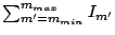 . Thus, Efficiency regarding the order
split is
. Thus, Efficiency regarding the order
split is
![\begin{displaymath}
\frac{I_m}{I_{total}} = \frac{
\frac{d'}{d} \frac{2}{(kd'E...
...}
\frac{d'}{d} \frac{2}{(kd'E_{m'})^2} (1-\cos[kd'E_{m'}])
}
\end{displaymath}](img230.png) |
(64) |
From Equation 10, emergent angle depends on both
and when and are fixed. When taking spectra of a
wavelength band from  through
  , we have to
be careful not to allow the light from the next orders (
, we have to
be careful not to allow the light from the next orders ( ) into
the observed . For this, following condition has to be satisfied:
) into
the observed . For this, following condition has to be satisfied:
 |
(65) |
Table 1 shows the allowed for the NIR bands when
we want to take spectra of the whole band at once.
Table 1:
Allowed orders of diffraction with spectra not overlapping.
| Band |
( ) ) |
() |
allowed orders |
 |
1.13 |
1.37 |
-5  5 5 |
 |
1.50 |
1.80 |
-5 5 |
|
2.01 |
2.42 |
-5 5 |
|
Figures 4 - 9 shows the results from calculation in
the Excel file for J-band and K-band gratings.
It turned out that:
- Lower order has higher efficiency.
- Better efficiency can be achieved when and
have the same sign.
- Incident angle and emergent angle should be as near as possible.
- Grating constant should be as big as possible.
All the results indicates that we get better efficiency with bigger
optics.
Figure 4:
Efficiency of the J-band grating plotted for emergent angle.
 ,
,
 optimized for
 with
with
 .
.
|
|
Figure 5:
Efficiency of the J-band grating plotted for wavelength.
,
optimized for
with
.
|
|
Figure 6:
Slit function for different orders with
 and
and  . Squares and circles indicates the integer orders
which angles light of
. Squares and circles indicates the integer orders
which angles light of  actually emitted. For the
configuration, integer order exists in the wing of
the primary peak of slit function, which makes the efficiency worth.
actually emitted. For the
configuration, integer order exists in the wing of
the primary peak of slit function, which makes the efficiency worth.
|
|
Figure 7:
Change of efficiency in different orders for K-band grating.
 ,
,
 ,
,
|
|
Figure 8:
Change of efficiency in different
 for the K-band grating. ,
  .
.
|
|
Figure 9:
Efficiency dependence on groove interval for the K-band
grating.
 , .
, .
|
|
Derivation of and from
Equation 12 is derived to satisfy the following conditions.
 |
(66) |
From
 ,
,
 .When we define
 and
and
 ,
,
because
 . Therefore, the second
condition becomes
. Therefore, the second
condition becomes
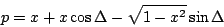 |
(70) |
and
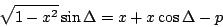 |
(71) |
Taking square of the both sides,
 |
(72) |
or
![\begin{displaymath}
0 = x^2[(1+\cos\Delta)^2+\sin^2\Delta] - 2p(1+\cos\Delta)x +
p^2-\sin^2\Delta
\end{displaymath}](img258.png) |
(73) |
When we define
 , an equation of the same shape
comes out. This means that the two solutions
, an equation of the same shape
comes out. This means that the two solutions  of the second
order equation corresponds to
of the second
order equation corresponds to  and
and  .
.
Solutions of Equation 74 are
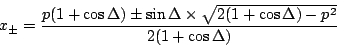 |
(74) |
Thus, and can be derived as  .
.
Following is a perl script to calculate and .
#!/usr/bin/perl -w

# subroutines
# arcsin from man perlfunc
sub asin { atan2($_[0], sqrt(1 - $_[0] * $_[0])) }

# usage
$usage = << '_USAGE';
usage: alphabeta.pl delta(deg) m d lambda
  with delta=|alpha-beta|, m=diffraction order, lambda=wavelength
  prints out solutions for alpha(deg) and beta(deg)
_USAGE

# Main routine
# usage
if (@ARGV != 4) {
  print $usage;
  exit -1;
}

# get command line options
$delta = shift(@ARGV);
$m = shift(@ARGV);
$d = shift(@ARGV);
$lambda = shift(@ARGV);

# calculation
$pi = atan2(1,1)*4;
$cosd = cos($delta*$pi/180);		# cos(delta)
$sind = sin($delta*$pi/180);		# sin(delta)
$p = $m*$lambda/$d;			# m*lambda/d
$p1 = (-$p*(1+$cosd)+$sind*sqrt(2*(1+$cosd)-$p*$p))/2/(1+$cosd);
$p2 = (-$p*(1+$cosd)-$sind*sqrt(2*(1+$cosd)-$p*$p))/2/(1+$cosd);
$a1 = asin($p1)*180/$pi;		# solution in degrees
$a2 = asin($p2)*180/$pi;		# solution in degrees

# results
print "$a1 $a2\n";
Original source of this document is at
siroan:~mos/design/010521_Grating/ and copied to
gin-an:~tomono/Presen01/010521_Grating/.
Revised version is edited at
gin-an:~tomono/Presen01/011228_Grating/.
Some of the plots are generated from
siroan:/win98/My Documents/tomono/Design01/Fiber/010514_OptTrain/SlitFunctions.xls.
HTML version of this document is posted at
http://www.rzg.mpg.de/~tomono/MOS/auth/Reports/011228_Grating/.
- 2001.5.23.
- -
- 2001.5.23.
- -
- Errata: parenthesis in Equation 4
- Another grating shape added (Figure 2(b),
Equations 61, and 62)
- 2001.5.24.
- -
- Derivation of and from
- Errata:
 coefficient in Equation 65
- 2001.5.28.
- -
- J-band grating
- Plots are updated according to change of Equation
- Second release
- calculation of
- 2001.12.21.
- -
- Source file copied to tomono@gin-an
- Link to the postscript file added to the html version
- Spell checked
- 2001.12.28.
- - Revised version
- Consideration of wide entrance slit
- 2002.1.10.
- -
- Equations 12 and 75 are corrected.
- 2002.1.11.
- -
- Perl script added for calculation of and .
- 2002.1.17.
- -
- 2002.2.4.
- -
Interferometry on a blazed grating
1
This document was generated using the
LaTeX2HTML translator Version 2K.1beta (1.52)
Copyright © 1993, 1994, 1995, 1996,
Nikos Drakos,
Computer Based Learning Unit, University of Leeds.
Copyright © 1997, 1998, 1999,
Ross Moore,
Mathematics Department, Macquarie University, Sydney.
The command line arguments were:
latex2html -dir html -mkdir -image_type png -local_icons -split 0 -up_url .. -up_title 'Parent directry' grating.tex
The translation was initiated by Daigo Tomono on 2002-02-04
Footnotes
- ... grating1
- Revised on December 2001.
Up: Parent directry
Daigo Tomono
2002-02-04
![$\displaystyle \frac{1}{N^2} \frac{1-\cos[kdNA']}{1-\cos[kdA']}$](img101.png)
![\includegraphics[width=0.8\textwidth]{nocoherent.eps}](img133.png)
![$\displaystyle \frac{\cos[\alpha_0]}{\cos\beta} \times \delta\alpha$](img150.png)

![$\displaystyle \frac{2d\cos[\alpha_0] \delta\alpha}{m}$](img153.png)


![$\displaystyle \frac{n\lambda_0 f_{col}}{\Delta s\cos[\alpha_0]}$](img200.png)
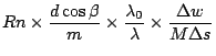
![$\displaystyle R n \times \frac{d}{m} \times \frac{\lambda_0}{\lambda} \times
\frac{\Delta w\cos\beta}{M\Delta s\cos[\alpha_0]}$](img201.png)
![$\displaystyle \frac{n\lambda_0 f_{col}\cos\beta}{\Delta s\cos[\alpha_0]}$](img203.png)
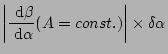
![$\displaystyle R n \times \frac{d\cos\beta}{m} \times \frac{\lambda_0}{\lambda} \times
\frac{\Delta w\cos\beta}{M\Delta s\cos[\alpha_0]}$](img204.png)
![\includegraphics[width=\textwidth]{J_orders.eps}](img241.png)
![\includegraphics[scale=0.5]{geometry.eps}](img29.png)

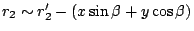
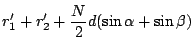
![$\displaystyle r'_1 + r'_2 - [\{(n-\frac{N}{2})d - \delta\}(\sin \alpha + \sin \beta)
+ \delta \tan \varepsilon (\cos \alpha + \cos \beta)]$](img53.png)
![$\displaystyle \sum_{n=0}^{N}\int_{0}^{d'} \exp[i\phi(\delta, n)] d\delta$](img63.png)
![$\displaystyle \sum_{n=0}^{N} \exp[-ikndA] \times \int_{0}^{d'} \exp[ik\delta E] d\delta$](img64.png)
![$\displaystyle \frac{1-\exp[-ikNdA]}{1-\exp[-ikdA]}
\times \frac{1}{ikE}(\exp[ikd'E] - 1)$](img65.png)
![$\displaystyle \int_{A_1}^{A_2} \frac{1}{N^2}\frac{1-\cos[kNdA]}{1-\cos[kdA]}
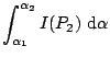
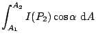
\frac{2}{(kd'E)^2} (1-\cos[kd'E]) \cos\alpha \mbox{ d}A$](img114.png)
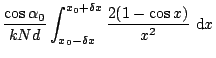
![$\displaystyle \cos\alpha_0 \int_{A'_1}^{A'_2} \frac{2(1-\cos[kNdA'])}{(kNdA')^2}
\mbox{ d}A'$](img124.png)
![$\displaystyle \frac{m\lambda}{2d\cos[\alpha_0] \delta\alpha}$](img157.png)


![\includegraphics[width=\textwidth]{J.eps}](img239.png)
![\includegraphics[width=\textwidth]{J_um.eps}](img240.png)
![\includegraphics[width=\textwidth]{Orders.eps}](img242.png)
![\includegraphics[width=\textwidth]{Delta.eps}](img243.png)
![\includegraphics[width=\textwidth]{d.eps}](img244.png)